Model the future. Explore the trade-offs and what-ifs.
Retire with confidence. Sleep well.
Financial planning at all levels involves navigation of some forbidding territory, but we’ve designed some unprecedented financial models to help you through it.
Trying to map out your financial plan? Struggling with some tough questions? Pralana Calculators can help!
Can I afford to switch to a lower-paying but more rewarding career? When can I retire? How much can I withdraw each year and still be confident that I won’t outlive my money? Do I need some supplemental income in retirement? How do I even go about building a financial plan? I’m not a financial expert; can I really do this myself? Is it worth my time to model the future in detail, particularly with so much uncertainty involved? After all, as someone famously said “It’s tough to make predictions, particularly about the future”.
The future is impossible to predict but Pralana Retirement Calculators have the ability to model in high fidelity the numerous interacting financial variables that will shape your future to help you gain a deep understanding of possible outcomes. Details matter if you want anything other than a rough approximation, and the Pralana Retirement Calculators can handle those details. They can be used effectively by anyone with a basic understanding of financial terminology such as inflation, assets and rates of return, and the motivation to dig in and do the work. They can help you answer the hard questions and make educated decisions. They can become your trusted companion.

Pralana offers three great retirement calculators and world-class support: Pralana Online is a web-based high-fidelity model similar to our Excel-based, downloadable Pralana Gold. Pralana Bronze is our free, Excel-based, downloadable calculator.
pralana online & and pralana gold
Pralana Online and Gold are much more than retirement calculators. They are personal financial models whose capabilities are unprecedented in tools primarily designed for personal use. Keep reading this page to learn more.
pralana bronze
Pralana Bronze is specially made for the person who wants to go beyond a quick-and-dirty financial analysis but prefers a simple, easy-to-use design. And it’s free!
user manuals
All our calculators are supplemented with detailed user manuals. The Online and Gold user manuals are so extensive that they may enlighten you on many key areas of retirement planning even if you don’t actually use the tool!
on-line support
The Pralana Retirement Calculator Forum enables users to help each other and share best practices. Further, the Pralana developer is always available for support.
Pralana Online and Pralana Gold are fully integrated, high-fidelity personal financial models that facilitate your execution of a robust financial planning process.

Begin by introducing yourself and your family, providing some basic assumptions, and then entering the details of your financial assets, income and expenses to establish a Base Plan. Then, you can do an initial analysis of your Base Plan to evaluate the viability of your plan based on the inputs you have provided, including the probability that you will not out-live your money. Depending on your analysis results, you might need to go back to the previous step and make some adjustments. If so, it is an easy process and once that is accomplished you can proceed to do various optimizations and refinements to establish your working plan. These can include variable spending strategies, optimization of your retirement age(s) and Social Security start age(s), detailed planning of Roth conversions and evaluation of your life insurance needs. Thereafter, it is easy to come back at any time to revisit and refine your plan and do further analysis.
Pralana Online and Pralana Gold have many powerful features that can be applied to planning your future
Here’s the 30,000-foot view…
High-fidelity modeling of income & expenses
Deals with the nuances of numerous types of income and expense streams and performs detailed Federal and State income tax and FICA tax calculations.
high-fidelity modeling of accounts & portfolios
Account-level rates of return are derived from user-specified asset classes and asset allocations
high-fidelity tabular and graphical projections
Tabular projections enable you to review what the tools are doing with your input data, and graphical projections put in easy-to-understand pictures.
Analysis & optimization
A range of likely outcomes is calculated by deterministic, Monte Carlo and historical analysis methods. These results can be enhanced with optimized Roth conversions, withdrawal order, Social Security start age and retirement start age calculations.
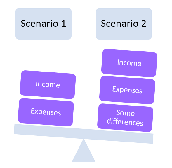
Pralana Online and Pralana Gold simultaneously model and compare three independent scenarios. This makes it a snap to study multiple options, trade-offs and what-ifs!
With their extensive modeling, analysis and presentation capabilities, Pralana Online and Pralana Gold can be powerful decision-making assistants. In mere minutes or even just seconds, they enable you to model different sets of assumptions and examine the long-term results. We refer to a set of income profiles, expenses profiles and assumptions as a “scenario”, and these Pralana tools allow you to define and model three independent scenarios simultaneously and then compare the results. Want to check out different life expectancies, different inflation rates, different asset allocations, different housing options, different retirement dates? No problem! Just copy your baseline scenario into one of the other scenarios with the click of a button and then modify the relevant fields, update your analysis, and do a side-by-side comparison. It’s truly that simple!
Some secrets of success
minimal use of simplifying assumptions
Most retirement calculators use numerous simplifying assumptions to make it easier on their developers, but each of those assumptions contributes to the error in the tool’s projections. Pralana calculators make a few assumptions also, but Pralana Online and Pralana Gold do not make many. The leading example is taxes: they make NO ASSUMPTIONS. They perform detailed Federal and State income tax and FICA tax calculations to completely eliminate that common and highly significant source of errors.
INTEGRATION OF COMPLEX INTERACTIONS
Some financial websites offer numerous free, independent calculators but offer nothing that models the real-world interactions between those operations. Pralana Online and Pralana Gold do it better! They are fully integrated models comprising hundreds of calculators and they model all of the interacting operations.
recognition that one size does not fit all
Pralana acknowledges that different users may have different preferences. Pralana Online is a high-fidelity, web-based tool that enables you to work on your plan anytime, anywhere, with all popular browsers. Pralana Gold is a high-fidelity tool that maintains your data on your local computer but is dependent on Microsoft Excel. Pralana Bronze is medium-fidelity tool that is free, simple to use, maintains your data on your local computer, and is also dependent on Excel. If you want to upgrade from Pralana Gold to Pralana Online, no problem: Pralana Online will import the data from Gold!
use of multiple platforms
Pralana’s downloadable calculators (Gold and Bronze) run equally well on Windows and Mac platforms. You can keep one copy on your home computer and another on your laptop, so you can work on your plan when you’re at home and when you’re away. Sharing data between the two copies is easy and Pralana calculators are kept current and are easy to update.
Testimonials
Don’t take our word for it; listen to what our customers are saying…
I love the many new features of Pralana Gold, especially being allowed to use specific dates instead of just years. I also love the addition of health care savings accounts and scheduled withdrawals from inherited IRAs. The earliest safe retirement date is a fun tool also. Wonderful product and the best value around – by a very, very wide margin!! Keep up the great, great work!!”
Paul R.
This is an amazing product that I’ve spent hours and hours utilizing to model my situation. I’m on the cusp of 60 and I read everything I see about personal finance. I’m a banker, MBA, so I know finance, and 99.99% of the time there is not much new. Your model is the best tool I’ve ever found!”
Mark H.
I’m thoroughly impressed with your work. It took me awhile with the user manual to work through the input and understand what the output was telling me, but it was a great exercise and learning experience. This will definitely provide the confidence we needed to proceed with our retirement.”
Mark M.
From the moment I found out about Pralana Gold from Darrow Kirkpatrick’s fine blog (Caniretireyet), I have been hooked on this great retirement calculator. It is superior in every respect to every other medium and high fidelity retirement calculator that I have used. The tool’s ability to effortlessly model various financial what-if scenarios with a holistic view of the results is truly invaluable (Roth conversion vs. no Roth conversion, moving from a high tax state to a lower-cost home in a low tax state, should I work part time or not?, should I pay off a rental property or not?, should I keep on working or retire now?, should I delay taking social security?, etc.). Additionally, Pralana Gold’s ability to do stress testing is exceptional (testing lower rates of return, higher inflation, longer life spans, higher expenses, etc.). And best of all the cost of Pralana Gold is miniscule – a heck of a bargain- and the support from the developer is truly excellent. I highly recommend this tool for young people all the way up to people in retirement, and for everyone in between. Fantastically useful, at a ridiculously low price.”
Shayne B.
I’m hooked! This is by far the most comprehensive of the 18 retirement calculators I tried and the easiest to use among the detailed ones. I started with the free Bronze version and loved it, so I bought Pralana/Gold and they’re in Excel so I don’t need to be online. It allows for impressive detail of inputs and variables, lets you easily test different scenarios, creates great reports, and gives this control freak everything I need. Customer service was prompt and thorough when I had questions. The User Guide is substantial and very useful, including examples. I have full confidence in its results!”
Catherine R.
I love this program, so powerful yet fairly easy to use! It has made our retirement planning much more a plan as opposed to a guess. I’ve endorsed it on Darrow Kirkpatrick’s website as well as with friends and relatives. And frankly, this is without a doubt the best $100 I have ever spent…for the price of a nice dinner out, getting to see where you’ll stand financially in the future based on where you are today…it really is a great bargain.”
Dwayne C.
Articles on Retirement Calculators
General Topics
Did you know that projections done with a fixed rate of return have roughly a 50% chance of being correct even if they’re based on a completely accurate average rate of return? Half the time those projections will be too low but the other half will be too high, and sometimes way too high.
We’re talking about “sequence of returns” errors. In the real world of investing, the return on your investments varies year by year and these variations affect the growth of your investments over the long haul. “Volatility” is a term used to describe and quantify these variations. The value of your investments at the end of the period will vary depending upon the cumulative effect of all the annual variations, even when the average of the annual returns over some period of years is constant. If you have a sequence of above-average returns early in the period, your investments will tend to fare better over the long run. On the other hand, if you have a sequence of below-average returns early in the period, your investments will tend to fare worse over the long run.
Monte Carlo and historic simulations create a large number of unique return sequences and apply them repetitively to your investments, then analyze the long term effects over the entire set of return sequences or what I call “the range of outcomes”. The Pralana calculators distill and present the range of outcomes in terms of percentiles, where any given percentile represents the value below which a certain percentage of the results fall. The Bronze calculator shows an envelope of results where the bottom of the envelope is the 10th percentile of results and the top of the envelope is the 90th percentile of results. The Gold calculator breaks the results down into a series of envelopes with each representing 10% of the results to give you much better insight into the distribution of results over the whole spectrum.

The solid red line near the center of the blue envelope is the projection based on a fixed rate of return over this 35-year period. The various blue bands around the red line are the distribution of Monte Carlo simulation results broken down into 10% groups.
The width of each band and of the entire envelope is a function of the expected volatility of your investments. If your money is in CD’s, volatility will be low and the envelope will be narrow. On the other hand, if a significant amount of your money is invested in stocks, volatility will be much greater and the envelope will be wide like the one shown here.
Projecting the future is impossible to do accurately but financial calculators employ one or more methods in attempting to do so. Projections that provide a single outcome based strictly on fixed rate returns have value in helping you gauge whether you’re heading in the right generation direction and in making choices between multiple financial options; however, users should be aware of their inherent limitations. Projections that provide a range of outcomes based on simulation of market volatility around user-specified averages or actual history (i.e., Monte Carlo or historical simulations) are imperfect too but have great value in giving you much better insights into how the future could unfold depending on the nature of your investments. This helps quantify the potential upside as well as the downside risk to better enable you to make decisions and give you more peace of mind. Even further, utilization of market volatility simulations in conjunction with consumption smoothing can be employed to establish your highest sustainable standard of living. The Pralana Gold calculator can do this!
The Dilemma for a Designer
In February 2017, Darrow Kirkpatrick (caniretireyet.com) posted an article describing a mysterious problem related to the size of the “time step” used by most retirement calculators in modeling decades of a user’s financial future. He pointed out that most calculators use years as their time step because using days, the time step unit of the real world, is impractical and then went on to elaborate on the potential modeling errors that could result from this design simplification. This article elaborates further on this issue and the practical solution that we developed in the course of our collaboration on this topic.
The dilemma Darrow described was in determining the “correct” way to sequence income, expenses and growth of accounts in modeling the increase and/or decrease of account balances over time. In the real world these are interwoven on a daily basis, but how to do this in a mathematical model that uses years as its time step wasn’t clear. One way to go is to apply the account growth at the start of the year based on its rate of return and balance at the end of the prior year, and then add/subtract income and expenses. Another way to go is to add/subtract income and expenses from the last year’s ending balance and then calculate growth based on that adjusted balance. On the test cases that Darrow used, he reported observing up to a 20% difference in the total long term projected account balance between these two methods of modeling account growth.
More Testing to Further Characterize the Problem
All models of the Pralana Retirement Calculator use the start-of-year growth algorithm but I became interested in the modeling errors this was introducing into long term projections when Darrow approached me with the dilemma he had encountered in his study. So, using a simple model of my own that implemented both methods of calculating account growth and a time step of years, I ran three tests cases: Case 1 involved a positive cash flow of $50,000 every year over a 40-year period, Case 2 involved a negative cash flow of $50,000 every year over a 40-year period, and Case 3 involved neutral (i.e., zero) cash flow every year over a 40-year period. I measured a 2.5% difference in ending balances between the two methods for Case 1 (long term positive cash flow), an 18% difference for Case 2 (long term negative cash flow) and 0% difference for Case 3 (neutral cash flow). (See the note below for an explanation of why case 2 exhibits a larger difference than case 1). I can now characterize the issue as follows:
The start-of-year growth algorithm understates long term projections (i.e., is too pessimistic) when positive cash flows are dominant and overstates those projections (i.e., is too optimistic) when negative cash flows are dominant
The end-of-year growth algorithm overstates long term projections when positive cash flows are dominant and understates those projections when negative cash flows are dominant, and this understatement can be quite significant
Cases 1 and 3 were not at all bothersome to me, but Case 2 is a definite concern. So, I decided to make the model more complex so that I could study the differences between the growth application methods using smaller time steps to get closer to the daily time steps in the real world. I elected to use months instead of years, so the model required 12 times as many calculations/steps but, as expected, it produced considerably smaller variations between the growth methods. Using the same test cases as described above, I measured less than 1% difference in ending balances between the two methods for Cases 1 and 3 and just under 2% difference for Case 2. We can readily conclude from these tests that the smaller the step size, the less it matters which growth method is used.
Note: Case 2 (negative cash flow) exhibits a much greater long term difference because the portion of the year-to-year account balance differences associated with the growth attributed to annual cash flow is much larger relative to the total year-to-year difference than with a positive cash flow of the same magnitude.
Solutions
Is the smaller step size the answer for retirement calculators? Before we can answer that we need to consider two things: 1) the practicality of using the smaller step size and 2) other alternatives.
Generally speaking, going from a step size of years down to months requires 12X the number of calculations and 12X the amount of time. Doing this for fixed rate projections is still no big deal; however, for Monte Carlo simulations which can involve hundreds or even thousands of scenario executions, this 12X factor can become significant indeed and could render the calculator to be impractical on many computer platforms. Still, a potential error in the range of 18% from just this one contributor is too large to ignore. There are other considerations and complexities associated with moving to a smaller time step size, but they’re beyond the scope and tangential to the point of this article.
What about other alternatives? Darrow and I discussed this and came up with one that retains the yearly step size while generating the same long term projection as a theoretical model with an infinitely small step size (all else being equal). This alternative applies growth in the middle of the year rather than at the start or the end. More precisely, the account balance at the end of the prior year is adjusted up/down based on half of the current-year cash flow, then a full year of growth is applied based on that mid-year account balance, and then the other half of the current-year cash flow is added. To evaluate this, I modified my simple model to implement this alternative. As expected, it produced long term results that were not affected by step size and that were always exactly half way between long term projections calculated using the start-of-year and end-of-year growth models regardless of step size.
This, then, allows me to reach this conclusion: Assuming that income and expenses are evenly distributed throughout the year, the mid-year growth algorithm results in the most accurate projection mathematically possible and the size of the time step is immaterial. Simply stated, it is more accurate than the other alternatives and more efficient in terms of calculations/ scenario than trying to increase accuracy by using smaller step sizes.
Incorporation into the Pralana Retirement Calculator
The mid-year growth algorithm is now part of PRC2017 and produces long term projections similar to my simple model when running the same three test cases; however, I’ve discovered that real world test cases can produce much more dramatic results. Darrow and I collaborated on the definition and evaluation of five realistic retirement test cases using PRC2017 Gold and his modeling framework. On four of these test cases our long term projections matched within 1% and within 5% on the fifth case using the start-of-year growth algorithm, so I’m confident of PRC results. At the time of our joint testing, Darrow hadn’t yet implemented the mid-year growth algorithm, so I went it alone in evaluating these same test cases with PRC. The differences between the start-of-year growth and mid-year growth algorithms was considerably more dramatic than I observed with the simple model and simple test cases described above. With our realistic test cases, I observed 11%, 9%, 0.5%, 1% and 21% differences! Note than PRC doesn’t and never has used the end-of-year growth algorithm, so I don’t have any related data.
I believe the mid-year growth algorithm in PRC2017 is more accurate than any alternatives in virtually every case while retaining the yearly step size to make it a practical solution on the typical computers of average users. PRC2017 still has the start-of-year growth algorithm, though, and allows users to specify which of the two growth algorithm options to use. Depending on your particular scenario, use of the mid-year growth algorithm may produce similar or significantly different long term projections. If you have a long period of negative cash flows, I strongly advise you to reanalyze your plan using this optimized algorithm.
Final Words
As of this writing, I have not yet identified the specific characteristics of the five realistic test cases that result in the much larger differences between start-of-year and mid-year growth algorithms as compared to those using the simple test cases. That’s a task for another day and the findings of that investigation will be reported when they’re available.
Retirement Calculator Design
This is a detailed, top-down technical article on retirement calculators. It has been prepared by the designer of the Pralana Retirement Calculator but it is written objectively and will not get into the subjective business of suggesting “the best retirement calculators”. Armed with the knowledge presented in this article, you will be equipped to assess for yourself the goodness of a retirement calculator and the extent to which it can be trusted to provide accurate and/or useful information, and then determine which one (s) might be “best” for YOU.
Retirement calculators are about one fundamental thing: they create a long term prognosis of your financial health based on certain assumptions and then allow you to change some or all of those assumptions to observe the effects on that prognosis. Here, in the simplest mathematical form possible, is the formula for creating that prognosis:
Long term prognosis = initial savings + growth of savings + deposits to savings – withdrawals from savings, projected out over your lifetime. The terms of this formula are defined as follows:
Growth of savings is often referred to as “rate of return” and is always expressed as a percentage. This percentage is then used to determine how the value of the savings accounts change each year, independent of any new contributions or withdrawals. For example, if the growth is 5%, then the size of the account at the end of year 2 will be 105% of what it was at the end of year 1 (ignoring the effects of inflation).
Your income, which is indirectly affected by inflation, includes wages, salaries, pensions, Social Security benefits, annuity payments, contributions made on your behalf by others (such as company-matching on your 401k contributions), windfalls such as inheritances, life insurance, or the selling of your home. Your expenses, which are usually directly affected by inflation, are every dime you spend, including payroll deductions, taxes, down payments on new property, house payments and utility bills, car payments and maintenance, gasoline, healthcare, college educations, food, clothes, vacations and so on. The difference between your income and your expenses determines whether you’re making deposits to or withdrawals from savings. Let’s call this difference ΔIE (delta IE, where delta refers to difference, I refers to income and E refers to expenses). When ΔIE is positive, you have a net deposit in the amount of ΔIE; when ΔIE is negative, you have a net withdrawal in the amount of ΔIE.
To create the projection of your savings, the retirement calculator simply has to do the following:
For the sake of this discussion, let’s say that savings accounts come in the following forms:
There are some issues that arise when trying to model these savings accounts in a retirement calculator:
The answers to the above questions have a direct bearing on the complexity of the calculator and on the complexity of the calculations the user has to perform just to make reasonable inputs to the calculator. These will be discussed below.
Calculating ΔIE, which is income minus expenses, is a simple thing once annual income and annual expenses are known; however, defining income and expenses involves some complexities and this is where we can find significant differences in the approaches used by the designers of retirement calculators.
As previously stated, your income includes wages, salaries, pensions, Social Security benefits, annuity payments, contributions made on your behalf by others (such as company-matching on your 401k contributions), windfalls such as inheritances, life insurance, or the selling of your home. One way or another, every retirement calculator must collect information from the user related to the various income streams and create an “income profile” that projects the user’s income into the future, including annual adjustments as appropriate.
As also previously stated, your expenses are every dime you spend, including payroll deductions, taxes, down payments on new property, house payments, healthcare, and college educations. One way or another, every retirement calculator must collect information from the user related to the various expense streams and create an “expense profile” that projects the user’s expenses into the future, including annual inflationary adjustments as appropriate.
Expense streams and, to a lesser extent, income streams, tend to be more complex during the accumulation phase than in the distribution phase because they include things like fixed rate mortgages which eventually get paid off, child-rearing/education expenses which taper off as the kids leave the nest, and company matching on contributions to 401k’s. To avoid this complexity, a common design choice is to treat the accumulation phase differently than the distribution phase. In this case, the calculator will not create income or expense streams during the accumulation phase and will instead simply ask the user to tell it ΔIE, (i.e., savings contributions during your working years). Armed with this number, all the calculator has to do is adjust it for inflation (or not) and add it to the growth-adjusted savings balance each year throughout the accumulation phase to create that portion of the calculator’s long term projection. Because the central focus of most of these tools is the retirement (or distribution) phase rather than accumulation phase, the vast majority of retirement calculators use this approach.
Moving ahead into the distribution phase, all retirement calculators actually perform the ΔIE calculation and use the user’s income- and expense-related inputs in doing so; however, there are large variations in the approaches used by retirement calculators in collecting these inputs. Approaches for collecting income vary from asking the user to specify Social Security and pension income to allowing the user to define multiple income streams for both husband and wife, including part-time employment or self-employment, Social Security, multiple pensions, annuities and windfalls. Approaches for collecting expenses range from asking the user to specify a single number representing total expenses for all time (commonly specified as a percentage of pre-retirement income) to specifying the details of a large variety of expense streams with variations over time, such as property, child-rearing, healthcare and discretionary expenses.
A complicating factor intentionally omitted from the discussion on calculating ΔIE is taxes, specifically income and FICA taxes. Taxes are an expense, but there is no standard way for treating taxes in the world of retirement calculators. Here are some of the approaches in use:
This disparity in the handling of taxes is one of the reasons why you can observe very different results from various calculators to seemingly the same input data. The next article will clearly explain why the different approaches yield different outputs and quantitatively address the sensitivity of long term projections to errors in tax calculations.
As a quick review, we’ve now discussed the growth of savings and the calculation of deposits to and withdrawals from savings, including the effects of taxes. Let’s now turn our attention to keeping track of your savings as it grows or declines and as we make deposits and withdrawals.
If the calculator treats all savings as one common pool and simply doesn’t try to model the unique characteristics of separate types of savings, then all it has to do is add annual ΔIE to the old balance to get the new balance. A subset of these calculators recognize that withdrawals from savings can be a taxable event and apply a tax burden on all withdrawals based on the user-supplied tax rate.
The calculators that manage the various savings accounts separately must deal with considerably more complexity than those that model savings as a single pool of money. In these calculators, a positive ΔIE is probably treated as a deposit to regular savings but when ΔIE is negative these calculators must determine which account to take the withdrawal from. The order in which withdrawals are taken across the various savings types may or may not be under the user’s control. A common approach would be to take it from regular savings first and when that’s depleted, then go to either tax-deferred or tax-free accounts to cover the deficit. In any case, the calculator must establish the order in which withdrawals are to be taken whenever negative cash flow (negative ΔIE) situations occur and it must work its way from one account to the other whenever the withdrawals result in the depletion of one or more of the accounts (possibly when negative ΔIE is large and prolonged over several years). When this process results in withdrawals from tax-deferred savings, this is a taxable event which in turn affects expenses. When this process results in withdrawals from regular savings, this may be a taxable event with an attendant effect on expenses. It depends upon whether the growth of the regular savings is taxable as simple interest/dividends (taxable annually as the growth occurs) or taxable as long term capital gains (taxable only when withdrawals are made and then only on the growth and not on the principle). Some calculators have the capability to fully model this while others always assume growth is to be treated as simple interest.
Calculators that keep track of the balance of tax-deferred accounts typically also deal with the issue of Required Minimum Distributions (RMD’s) and automatically generate taxable withdrawals starting at age 70 or 71. These RMD’s can be treated as additional income or as additional deposits to regular savings. Regardless, the RMD’s must be accounted for in the process of keeping track of the balances of the various types of savings accounts. They matter because they’re a taxable event which has ramifications on annual expenses.
So, here’s a simple question to ponder: Presumably there are financial advantages and disadvantages to regular accounts vs. tax-deferred accounts vs. tax-free accounts and it makes a significant enough difference for us to employ different accounts in preparing for retirement; otherwise, we’d just put all our money in one account and not worry about it. Does a similar consideration come into play when it comes to modeling our savings over time in a retirement calculator? Does trying to model the complexity described above actually matter when it comes to a prognosis of your financial future? Think about it and we’ll come back to it in the discussion of Pooled vs Separate Savings Accounts.
This discussion is moot if you’re already retired or quickly approaching retirement. Otherwise, it might be pertinent to you. The reason it matters is that the accuracy of your portfolio estimate at the start of your retirement is a function of how accurately your accumulation phase is modeled. Inaccuracies in this estimate will then be magnified over the distribution period because of the law of compounded returns.
To be clear on the terminology, the accumulation phase generally refers to your pre-retirement years when you’re building your savings and the distribution phase generally refers to your retirement years when you’re making withdrawals from your savings to cover retirement expenses. Regarding the modeling of these phases, retirement calculators tend to fall into one of two categories:
To get specific about potential difficulties in determining a single value representing ΔIE, here are a few examples of expenses that are likely to occur during the accumulation period which can make it difficult to come up with a good average annual contribution amount:
You may be thinking that inputting ΔIE directly is ideal because that allows you to set up the calculator to be consistent with your real-world payroll deductions for contributions to savings. There are two major issues with this:
Clearly, then, errors will be introduced into a calculator’s prognosis whenever it asks the user to specify the average savings contributions per year and if, over time, that number isn’t consistent with the expected difference between income and expenses. Check out the table below to get a feel for the effect of this type of error. It shows how errors in savings contributions to taxable savings during a 15-year accumulation period would be magnified during retirement periods of 20 and 30 years, including the effects of taxes.

So, an input error of only $1000 per year for 15 years will lead to a 4% error in the portfolio’s ending value after a 30-year retirement, but an input error averaging $5000 for a 15-year accumulation period will lead to a 20% error after a 30-year retirement.
In the final analysis, this may or may not matter to you depending upon your circumstances and what you want to achieve with the retirement calculator. It doesn’t matter at all if you’re already retired or are nearing retirement. It probably won’t matter too much if you’ve adopted a repetitive approximation approach for evaluating retirement readiness wherein you take a quick look once in a while with your latest numbers. It may matter a lot if you’ve still got a long way to go to retirement and are using the calculator to assist you in evaluating the long term financial impacts of multiple lifestyle alternatives.
As a quick refresher, we’ve defined the term ΔIE to be the difference between income and expenses and have stated that a positive value represents a positive cash flow and net deposits to savings while a negative value represents a negative cash flow and net withdrawals from savings. Some retirement calculators use the term “retirement income requirements”, but what they’re really talking about are your expenses in the distribution phase.
Regardless of the terminology used to refer to expenses, this is another area where we can differentiate low fidelity from high fidelity calculators. Many calculators only allow expenses to be defined by a single summary-level value while others allow for expenses to be defined to whatever level of detail the user desires. Some of the latter category of calculators go so far as to model college educations, home mortgages and other property-related expenses, healthcare expenses that vary greatly from early to late retirement, one-time expenses, and so on. Clearly, the first group of calculators belongs to the low fidelity category while the second group meets at least one important criterion for a high fidelity calculator.
There are rules of thumb suggesting that retirement income requirements (i.e, expenses during your retirement years) should be assumed to be a particular percentage of your pre-retirement income, and many retirement calculators ask for your input in those terms. The author of this article considers that to be complete nonsense and will not propagate any such numbers here. Unless you’ve continually raised your standard of living to keep up with your income throughout your working years, your expenses in retirement will not necessarily be a high percentage of your income at the time you retire. The fact is that the only way to know what your retirement-era expenses are going to be is to figure it out, then review and update it from time to time. As a starting point, you can look at your current expenses and determine which of them you’ll still have after you retire and for how long, and quantify them in terms of today’s dollars. If you plan to downsize your home, write that down along with the related details. If you plan to take up new activities, maybe you need to add an expense item or two.
With that said, there are really two fundamental ways of going about this:
You may be of the opinion that it’s a waste of time to attempt to model taxes because we don’t know what Uncle Sam is going to do to tax rates in the future. I believe the correct approach is to use the best information available (i.e., the current tax code) to establish a baseline plan, supplement that with a sensitivity analysis based on potential future tax increases, and then revisit your analysis from time to time to make updates based on any new information that has become available.
With that said, retirement calculators generally fall into one of three tax-handling categories: 1) those that perform detailed tax calculations, 2) those that account for taxes based on user-specified tax rates and 3) those that ignore taxes. If you go with one of those that perform detailed tax calculations, you simply do not have to concern yourself with taxes and can be reasonably confident that they’re being accounted for accurately. If you go with one of those that estimate taxes based on user-specified tax rates, then you have to accurately determine the proper tax rate to use and how it might vary over time and enter that into the tool, knowing that most tools only accept a single rate that applies to the entire modeling period. Finally, with the set of tools that ignores taxes altogether, you can either choose to ignore taxes yourself, or you can figure your tax rate and then manually adjust your income and expense inputs to the tool to account for taxes.
The first set of tools (those that perform detailed tax calculations) requires you to do no tax-related math yourself. The next set requires you to determine your income tax rate and/or your investment tax rate for your working years, early and late retirement years and then, for most calculators, boil them down to a single average value. The last set requires you to do everything the second set does in addition to using that value to adjust all of your income and expense values. So, not only do you have to do more work in the second and third cases, but there’s also increased risk of error.
Going back to the subject of performing a sensitivity analysis on tax rates, some calculators make this easier and less error prone than others and fall into one of two categories: 1) those that allow you to specify tax rate changes at specific times in the future and 2) those that use the same tax rate across the whole modeling period or ignore taxes altogether. If you use one of the latter set, you will have less control over your analysis and will have to do more work yourself. In the Calculator Evaluation article on this website, four of the five tools in the High Fidelity set perform detailed tax calculations AND allow you to specify future tax rate increases (amount and date), as well as decreases in Social Security benefits. The fifth tool (Flexible Retirement Planner) doesn’t do detailed tax calculations but it does allow you to specify both income and investment tax rates (and Social Security benefits) on a year by year basis if you so choose.
Ignoring ease-of-use issues and user-induced errors, I decided to do some testing to try to quantify the affect different tax-handling approaches might have on calculator outputs. To get the absolute best apples-to-apples test I could, I used just one calculator (Flexible Retirement Planner – FRP) and then modeled taxes using three different approaches for the distribution period (all approaches were identical for the accumulation period): Approach 1) with several periods of different tax rates, with rates as measured by the Pralana Retirement Calculator (PRC) which performs detailed tax calculations, Approach 2) with a constant tax rate, using the average measured by PRC and Approach 3) with tax rate set to zero and income and expenses adjusted to compensate for taxes, again using the average tax rate as measured by PRC. Using only test case 1 defined in the Calculator Evaluation article (60 year-old couple beginning a 40-year retirement with $1,100,000 and $24,000 of Social Security income starting at age 66) and with all other parameters exactly the same for each tax-handling approach being evaluated, here are the final savings balances (in today’s $) I observed:
Observation #1: there was only a 3% error introduced by using a constant tax rate rather than a nuanced tax rate.
Observation #2: if you manually compensate for taxes by adjusting income and expenses, the errors are worsened if there are periods where you actually pay no taxes, such as the first several years of Case 1 where all expenses are covered by withdrawals from taxable savings. So, in this case, expenses are exaggerated by modeling taxes which may not actually have to be paid.
Observation #3: Even though the exact same average tax rate was used for approaches 2 and 3, substantial differences in the final savings balances were projected. There are two reasons for this:
I repeated this tax analysis using Case 2 (involving both accumulation and distribution periods) and got similar results and for the same reasons:
Conclusions:
Finally, I decided to do one more test. Conclusion #2 above says it doesn’t make much difference whether you use a flat tax rate or a more nuanced one; however, it doesn’t say anything about user-induced errors in the specification of those flat tax rates. So, for this test, I again used FRP and the test case 1 scenario, but with three different tax rates: 8%, 9% and 10%. Final savings balances were as follows:
Conclusion: Absolute precision in specification of your tax rate is not crucial; however, just making a rough estimate will probably result in substantial errors. For this test case, it appears that each 1% error in tax rate results in an 8% error in the final savings balance. This error is avoidable by using a calculator that performs detailed tax calculations.
Previously, a question was posed on whether it makes a significant difference whether a retirement calculator models savings accounts separately according to their unique characteristics or simply models them as a common pool. The test case described below, involving only the distribution phase, is enlightening. In this case, there’s $1,000,000 in savings at the start of a 30-year retirement that begins at age 65, and retirement expenses are about twice the retirement income such that withdrawals from savings will be made throughout the retirement years. The exercise here is to study the differences in the final savings balance with respect to variations in how the $1M is split between tax-deferred, Roth and taxable savings accounts, and the extent to which the growth of taxable savings is due to simple interest or capital gains (which affects its taxation). This test was performed using the Pralana Retirement Calculator (Gold version) which performs detailed federal income tax calculations with no tax rate inputs from the user. The rate of return is the same on all accounts. Taxable account balances go above zero despite a zero initial balance due to RMD’s. The details are presented in the table below, in today’s dollars.

We can readily conclude from this data that there are significant differences in final account balances depending on whether the calculator models separate savings accounts or simply treats them as a common pool. We can see up to 19% variation depending simply upon whether the growth of regular savings is simple interest or capital gains (see the case where the $1M is split between tax-deferred and taxable savings at the start of retirement). Additionally, we can see up to 18% variation depending upon how the money is split between the various accounts at the start of retirement even with no variation in whether the growth of regular savings is simple interest or capital gains.
In real world investing, we choose to put money in different types of accounts because it really does matter, and these findings indicate that it matters in the world of modeling as well.
Most free retirement calculators are truly easy to use once you’ve done your homework and have translated all of your financial details into the form they’re expecting. This commonly boils down to annual contributions to savings, annual income during your retirement years and when it will begin, your retirement income requirements (i.e., retirement expenses), tax rate, rate of return on savings, inflation rate and life expectancy. Armed with these numbers, it’s usually a simple matter to plug them into the calculator and get quick results.
Retirement calculators do the math that integrates the data described above into a long term projection. That’s difficult for most people to do on their own and, hence, retirement calculators can be useful tools. The rest of the story, though, is the downside of the statement “once you’ve done your homework and have translated all of your financial details into the form they’re expecting”. Let’s briefly consider some of the inputs required:
In contrast to the above, some high-end retirement calculators provide much more robust data input capabilities that allow you to characterize your financial situation in rich detail while eliminating the need for you to do most or all of the “off-line” math required by the low-end calculators. This actually makes your job quite a bit easier and it reduces the opportunities for math errors; however, to be completely fair and depending upon the calculator, more robust data input capabilities makes for a more complicated user interface and creates opportunities for misinterpretation of the inputs being requested by the calculator. This, then, accentuates the need for a quality user manual to accompany any complex calculator.
One or more of the following analysis methods are employed by all retirement calculators to produce their outputs:
Each of these analysis methods offer some goodness but none of them is perfect. Therefore, the more information you can gather and the more different methods you can employ to examine your financial future, the better equipped you’ll be for making decisions.
No calculator can forecast the future with certainty because the calculations are always based on assumptions related to certain variables that are unknowable in advance, and this translates into some degree of risk in relying on their predictions.
Topping the list of unknowns are:
The primary risk areas are then:
There’s little you can do about any of these unknowns, but it can be useful to understand where the associated risks lie and how sensitive your financial plan is to variations in key variables. That’s where a trustworthy retirement calculator can help:
We’re all affected by things beyond our control, such as inflation, government policy (e.g., tax rates, Social Security benefits), the rising cost of healthcare and the volatility of certain investments. But we also face many decisions in life which are largely under our control. We weigh the pros and cons, make trade-offs, and try to assess how one decision interacts with other decisions. This includes job and career, getting married, having children, college educations for your children, housing choices, mortgages, how much to contribute to retirement accounts and what type of retirement accounts to have, healthcare, how much life insurance to carry, getting a divorce, when, where and how to retire, when to start collecting Social Security benefits, which survivor benefits to select with your defined benefits pension, long-term care, and on and on. The decisions we make on many of the above items have a direct bearing on our income stream and our taxes which, in turn, affect our discretionary spending power.
Then there are choices we have to make on discretionary spending such as vacations and travel, hobbies and entertainment, clothes, cars, luxury items, gifts and charitable giving. And, of course, there are also those non-discretionary expenses such as utilities, food and household items.
Without the right tools, putting all the pieces of the financial puzzle of our lives together is bewildering if not impossible. There may be other definitions of the term “life cycle calculator”, but I’m defining it to mean one that can model all of these types of things simultaneously and specifically including the modeling of various survivor scenarios. Further, a good life cycle calculator should also help the user establish an optimized standard of living. Suffice it to say that you will not get one of these in a free, on-line retirement calculator; however, you may find that these tools are worth every penny invested in them.
Consumption smoothing is a term used by economists to describe a consistent standard of living for an individual regardless of family size and the ebb and flow of non-discretionary expenses. In other words, it enables you to maintain the same level of discretionary spending (i.e., consumption) while you’re raising a family, paying your mortgage, paying for college educations, when you become empty nesters and when you’re retired. For reference, consumption smoothing is the subject of an excellent and easy-to-read book by Laurence Kotlikoff and Scott Burns entitled Spend ‘til the End. Consumption smoothing is mathematically complex and computationally intensive and is an extremely rare feature in retirement calculators. I’m aware of only two tools that provide a consumption smoothing capability: ESPlanner/MaxiFi and the Gold edition of the Pralana Retirement Calculator.
These tools can be very helpful in making lifestyle decisions, but you have to be careful in determining the level of trust to place on consumption-smoothed expenses. It’s one thing to get the calculations right, which isn’t easy, but it’s another thing to be able to count on them. Why? Because they’re subject to the same “unknowables” as all other projections: inflation, rates of return, life span, and so on. To reduce this risk, Kotlikoff and Burns suggest telling ESPlanner that you and your spouse plan to live to age 100. The Pralana Retirement Calculator takes risk reduction options to another level: it has the capability to utilize Monte Carlo and historical simulations in conjunction with consumption smoothing to calculate a standard of living with a 90% probability that your money will outlast you.
So, finally, I’m going to introduce the concept of a personal finance model (PFM) and then attempt to explain the power and convenience that such a tool can provide. A PFM should not be confused with personal finance software because those products tend to be money management and tax preparation tools. A PFM should be like a trusted friend that you can go to with virtually any issue, and here are some key phrases I’d associate with a good PFM:
If the tool makes sense to you, is sufficiently transparent that you can understand what it’s doing, is sufficiently flexible and robust to be able to model the nuances of your financial life, and you can understand and have confidence in what it’s telling you, then you have a tool that can become a trusted friend. Regular use of a well-designed tool will lead to familiarity, and that will lead to ease of use, convenience and even more confidence. Once you get to that point you’ll no longer have to “play the field”, trying to model your scenarios in various tools and trying to understand and normalize the differing outputs. Then you can get very quick turn-around on evaluating alternatives and what-ifs, and periodically updating your assumptions and reviewing long term projections for any warning signs. The tool will be there for you anytime you need it, and you’ll be comfortable with the process.
So, now let’s get specific about the characteristics of a good PFM. We’re really talking about way-high-end retirement calculators that meet the following requirements: